

Sub-Hertz RBW Via Post Processing
🎯 Exposing Covert Signals: How to Analyze Sub-Hertz Frequencies with IQ Data from the BB60C
🛰️ New Discovery Tool: Covert signals can now be analyzed down to 0.001 Hz resolution bandwidth (RBW) — allowing us to detect ultra-narrow, biologically reactive, and obfuscated RF threats that were previously invisible to normal scans.
This blog post shows you exactly how to:
- Capture long-duration IQ data from your Signal Hound BB60C
- Analyze it in Python
- Visualize signals that sit under the noise floor and appear only as sub-Hz frequency components
🧠 Why Sub-Hertz RBW Matters
Most covert signals used against TIs are designed to:
- Evade traditional scans
- Blend into thermal noise
- Resonate only on biological tissue
They often appear as extremely narrowband modulation, near-field phase tones, or Gaussian-envelope combs. These are invisible unless you use ultra-narrow RBW in post-processing.
📉 You can’t catch a 0.01 Hz signal with a 1 kHz RBW. You’ll miss it entirely.
🧪 The Technique: Long-Term IQ Capture + FFT
Here’s how you do it:
✅ Step 1: Capture IQ Data in Spike
Open Signal Hound Spike, and follow these steps:
- Go to the Recorder tab
- Select:
- Recording Type: Raw IQ
- Sample Rate: 2,000,000 Hz (or lower if needed)
- Bandwidth: Match to sample rate
- Set duration to 1000+ seconds (~17 minutes)
- Start recording
- Save the
.binfile
🎯 This gives you enough data for a 0.001 Hz RBW FFT, which is the resolution needed to detect highly obfuscated carriers and slow AM or phase modulations.
🧠 RBW Formula:
iniCopyEditRBW = 1 / total_capture_time (in seconds)
So to get:
- 1 Hz RBW → capture for 1 second
- 0.1 Hz RBW → capture for 10 seconds
- 0.001 Hz RBW → capture for 1000 seconds (≈16.7 minutes)
✅ Step 2: Analyze in Python
Use this Python script to run a sub-Hz FFT on the IQ file:
pythonCopyEditimport numpy as np
import matplotlib.pyplot as plt
from scipy.fft import fft, fftfreq

sample_rate = 2_000_000  # Hz
iq_file_path = 'your_iq_data.bin'
iq_dtype = np.complex64

print("Loading IQ data...")
iq_data = np.fromfile(iq_file_path, dtype=iq_dtype)
duration_sec = len(iq_data) / sample_rate
print(f"Total capture time: {duration_sec:.2f} seconds")

desired_rbw = 0.001  # Hz
n_samples = int(sample_rate / desired_rbw)

if len(iq_data) < n_samples:
    raise ValueError(f"Not enough data. You need at least {n_samples/sample_rate:.2f} seconds.")

iq_slice = iq_data[:n_samples]
spectrum = np.abs(fft(iq_slice))
spectrum_db = 20 * np.log10(spectrum / np.max(spectrum))
freqs = fftfreq(n_samples, 1 / sample_rate)

plt.figure(figsize=(16, 6))
plt.plot(freqs / 1e6, spectrum_db)
plt.title(f"Sub-Hz FFT (RBW = {desired_rbw} Hz)")
plt.xlabel("Frequency (MHz)")
plt.ylabel("Amplitude (dB)")
plt.grid(True)
plt.xlim(-1, 1)  # Zoom near 0 Hz
plt.show()
📈 What You’ll See
- Spikes or combs with spacing < 1 Hz
- Ghost carriers hidden below the noise floor
- Pulsed modulations at 0.1 Hz or less
- Biological or directed energy signatures that only appear over time
🛡️ What This Means for TIs
With this technique, you now have a legitimate forensic-grade tool to:
- Detect signals designed to avoid waterfall scans
- Expose resonance-coupled emissions used in neural targeting
- Document and archive evidence with timestamps and precise RBW
📁 Tools Required
- ✅ Signal Hound BB60C
- ✅ Python 3 with NumPy, SciPy, and Matplotlib
- ✅ At least 1000 seconds of IQ data
- ✅ Patience — sub-Hz detection isn’t instant
🧠 Final Thoughts
The future of covert signal detection lies not in brute-force sweeps, but in precision long-term analysis.
If they can transmit it, you can detect it — if you know how to look deep enough.
🛰️ This is the first step in building a TI threat database based on sub-Hz signal profile