Sunday, 08 June 2025 / Published in Signal Intelligence & Detection Techniques

Cyclostationary Analysis

Spread the love

🧠 Cyclostationary Analysis in Signal Intelligence: A TI-Friendly Tutorial

🔍 What Is Cyclostationary Analysis?

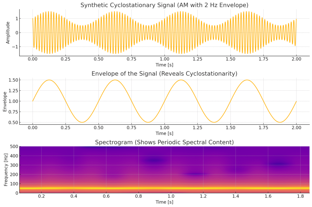
Cyclostationary analysis is a powerful tool in signal intelligence (SIGINT) used to detect and classify repetitive, structured patterns in electromagnetic signals, especially those designed to hide in noisy environments.

Unlike a basic spectrum analyzer — which only shows how much energy is present at a frequency — cyclostationary analysis looks for periodic statistical features that indicate modulation, timing, or intentional structure.

📡 Why It Matters for Targeted Individuals

Many TIs report harassment involving unknown electromagnetic signals or covert communication systems. These signals may:

Appear only intermittently
Be embedded under noise
Use spread-spectrum or backscatter techniques
Avoid detection by standard spectrum analyzers

Cyclostationary analysis is specifically designed to detect signals that are deliberately masked — making it a useful tool in cases where normal RF sweeps show nothing, but interference, symptoms, or effects persist.

🧠 Is Cyclostationarity Used in Implant Systems?

There is no direct public evidence proving that brain implants or nano-devices use cyclostationary modulation themselves — but here’s the key:

Many covert communication systems — like RFID, neural telemetry, and LPI radios — do use modulation techniques that create cyclostationary patterns.

This includes:

Clocked load modulation (used in RFID and passive implants)
Chirp spread spectrum (used in LoRa and implant telemetry)
Phase/frequency shift keying (common in secure comms)
Burst gating and time-domain multiplexing

These techniques all produce repetitive features that cyclostationary tools can detect.

So while we can’t say “implants use SCF” — we can say:

“If a covert device is transmitting, and it’s using known modulation or backscatter techniques, SCF is one of the few methods that can find it.”

🔬 How Cyclostationary Analysis Works (Step-by-Step)

Input: IQ Data
- You start with raw .iq files from an SDR like a HackRF, LimeSDR, or Signal Hound BB60C.
Preprocessing: Filtering + Windowing
- Apply bandpass filters to isolate the frequency band of interest.
- Divide the signal into overlapping windows for statistical analysis.
SCF Computation
- For each frequency f and cyclic frequency α, compute how much energy repeats every 1/α seconds.
Visualization: Spectral Correlation Plot
- The result is a 2D heatmap where vertical structures show strong periodicity — a hallmark of modulation.
Interpretation
- Repeating structures ≠ random noise.
- If you see line pairs, symmetry, or peaks in the alpha domain, it indicates modulation — even if the signal looks like noise on a spectrogram.

💻 Example Code (Python)

pythonCopyEditfrom demod import compute_cyclostationary_scf, plot_scf
import numpy as np

# Load your IQ data (e.g., from raw.iq)
iq_data = load_iq_file("raw.iq")
fs = 20e6  # Sampling rate

# SCF alpha range
alpha_range = np.linspace(-1e6, 1e6, 50)

# Run SCF
scf, freqs, alphas = compute_cyclostationary_scf(iq_data, fs, alpha_range)

# Save or view the plot
plot_scf(scf, freqs, alphas, output_file="output/scf_plot.png")

🛡️ When to Use SCF in a TI Scan

Situation	Should You Use SCF?
Basic Wi-Fi or cell tower detection	❌ No
Suspected backscatter communication	✅ Yes
Short burst, noise-hidden RF signals	✅ Yes
Periodic signals causing V2K or Frey-like effects	✅ Yes
Implant telemetry suspected	⚠️ Possibly — SCF may help detect structure

📚 References

Gardner, W. A. Cyclostationarity in Communications and Signal Processing, IEEE Press, 1994
“Backscatter Communications for Implantable Devices,” IEEE Access, 2019
“Clocked Load Modulation for RFID,” Radioengineering Journal, 2017
US Patent 6470214B1 – Apparatus and method for remotely monitoring and altering brain waves
US Patent 6011991A – Communication system and method including brain wave analysis

✅ Final Word

If you’re doing serious RF forensics as a targeted individual, tools like SCF give you a real edge. It’s not about guesswork — it’s about picking up patterns that covert systems can’t easily hide.

The signal might not be strong.
The signal might not be wide.
But if it’s structured, SCF will see it.

🚫 Why Cyclostationary Analysis Fails Without Proper Equipment

1. Insufficient Noise Floor (Sensitivity)

Cyclostationary analysis depends on detecting subtle repetitive patterns, often buried under ambient noise.

If your device’s noise floor is too high — meaning it can’t distinguish between signal and background noise — then:

The signal is masked completely
The SCF (spectral correlation function) matrix becomes noisy
No reliable structure can be extracted

📉 Think of trying to hear a whisper at a rock concert — SCF is only helpful if the “whisper” is above the system’s minimum discernible signal (MDS).

2. Poor Resolution Bandwidth (RBW)

To identify modulation signatures or narrowband combs:

You need very fine resolution bandwidths (RBW), often in the sub-kHz or even Hz range
SDRs like RTL-SDR may have RBW in the tens or hundreds of kHz — too coarse for this task

💡 Professional equipment like the Signal Hound BB60C, RSA500 series, or Rigol RSA3000 allows for fine-grained RBW down to 1 Hz or better — essential for detecting narrow comb teeth or low-rate modulations.

3. Aliasing and Sampling Rate Issues

If the sampling rate is too low, signals of interest may alias into false patterns or be filtered out entirely.
For high-frequency combs (like 1.33 GHz ± 240 kHz), you need to sample at ≥ 2.66 GHz for direct capture — or use downconversion + heterodyning.

📦 SCF relies on accurate temporal periodicity, so timing artifacts introduced by cheap ADCs (analog-to-digital converters) can completely destroy analysis integrity.

4. Short Capture Duration

If your capture window is too short, there’s not enough data to statistically confirm a cyclostationary feature.
Many modulations (like DSSS or burst-gated signals) need several seconds or minutes of data to accumulate SCF features.

⏳ The longer your IQ sample, the stronger the SCF features become — assuming your equipment can maintain stable timing.

✅ Minimum Equipment Requirements for Reliable SCF in TI Investigations

Spec	Minimum Requirement
Noise Floor	≤ -120 dBm (ideally lower)
RBW	≤ 1 kHz (ideally sub-Hz)
Sample Rate	≥ 20 MHz (for downconversion)
Storage	≥ 1–5 GB for long IQ captures
SDR	Signal Hound BB60C, RSA500, LimeSDR (limited), HackRF (borderline)
Antenna	Tuned, directional, low-noise preamp

🧠 Summary

Cyclostationary theory is powerful — but only when your tools are good enough to see below the surface.

You can have perfect software, the right code, and the most detailed processing — but if your gear can’t see it, you’re blind to the attack.